The Discrete Fourier Transform

The Discrete Time Fourier Transform

Consider a discrete time signal . Its discrete time Fourier transform (DTFT) is given by,

And its inverse is given by,

The DTFT calculates the frequency spectrum of a discrete-time signal. Its result is continuous in frequency as well as periodic.

The Discrete Fourier Transform

The DTFT can not directly be computed by a computer as it requires the calculation of an infinite summation. Discrete Fourier transform (DFT) resolves this problem by assuming a finite length signal.

Let be non-zero only for . Then, the DTFT can be computed as,

Since, the time domain consists of only samples, the frequency domain will also have only independent samples,

where, , .

Equation is the DFT, and its inverse is given by,

The DFT matrix

For points, the DFT represents the data using sine and cosine functions with integer multiples of a fundamental frequency in the twiddle factor, .

From , it can be observed that the DFT is a linear operator which maps data points in spatial domain to in frequency domain.

where, the DFT matrix is a unitary Vandermonde matrix.

The output vector contains the Fourier coefficients for the input vector .

The 2-Dimensional Discrete Fourier Transform

The 2D DFT can then be given as,

And its inverse as,

The 2D DFT can be viewed as a sequence of two 1D DFT applied to the first variable and then the second. In case of image, this means applying a 1D DFT along the column and then applying another 1D DFT along the row of the result obtained from the first transform.

The Implementation

Let us first import the libraries that we will be using.

import numpy as np
import plotly.express as px
import requests

from PIL import Image

Using DTFT Matrix

From , it can be observed that the DFT can be computed if we can compute . The code to compute it is given below:

def dft_matrix(N: int = 256):
    w = np.exp(-2 * np.pi * 1.j / N)

    j, k = np.meshgrid(np.arange(N), np.arange(N))
    W = np.power(w, j * k)
    return W

If we visualize the real part of for , then we obtain:

W_512 = DFT_matrix(N=512)

px.imshow(np.real(W_512), width=600, height=600)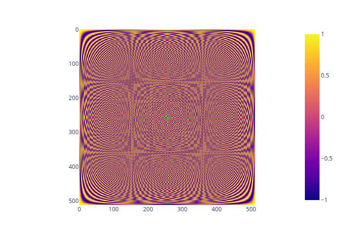

Now, the 1D DFT can be implemented as,

def dft(x):
    W = dft_matrix(x.shape[-1])
    return W @ x

And the 2D DFT can be implemented as,

def dft2(x):
    W = DFT_matrix(x.shape[-1])
    X = W @ x
    W = DFT_matrix(x.shape[-2])
    return (W @ X.T).T

Now, let’s apply our implementation to perform the discrete Fourier transform. For this we need to obtain an image first

url = "https://c02.purpledshub.com/uploads/sites/48/2024/04/helix-nebula.jpg"
img = Image.open(requests.get(url, stream=True).raw).convert("L").resize((512, 512))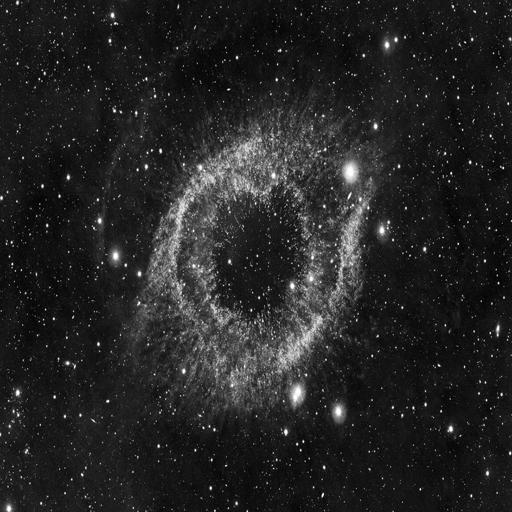

Now, we can apply the discrete Fourier transform on it

img_np = np.array(img)
img_dft2 = dft2(img_np)

Let us check that our implementation is correct by comparing it with the fast fourier transform provided by numpy.

img_fft2 = np.fft.fft2(img_np)
print(np.isclose(img_dft2, img_fft2).all())

The above code results in the following output

np.True_

This means that our implementation is correct.

Let us visualize the transformed image.

plt.imshow(np.log(np.abs(img_dft2)**2))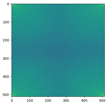

Based on our current implementation, the frequencies [0, 0] is at the top left corner. Centering the Fourier transform can make it easier to interpret the frequency content of the image. However, to center the transform, we require negative frequency components. So, where are these negative frequency components? The second half of the frequency components are the negative frequency components.

def dftshift(x, axes=None):
    if axes is None:
        axes = tuple(range(x.ndim))
        shift = [dim // 2 for dim in x.shape]
    elif isinstance(axes, integer_types):
        shift = x.shape[axes] // 2
    else:
        shift = [x.shape[ax] // 2 for ax in axes]

    return np.roll(x, shift, axes)

Now, the fourier transform of the image can be centered as,

shifted_img_dft2 = dftshift(img_dft2)
plt.imshow(np.log(np.abs(shifted_img_dft2)**2))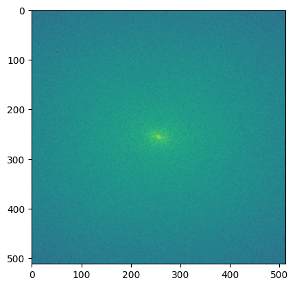

Using Basis Images

Equation can be written as,

The exponential part in the above equation forms the basis image for horizontal and vertical frequency when evaluated at each pixel coordinates

def dft_basis_2d(N: int, M: int, u: int, v: int):
    n, m = np.meshgrid(np.arange(0, N), np.arange(0, M), indexing="ij")
    return np.exp(-1.j * 2 * np.pi * (n * u / N + m * v / M), dtype=np.complex128)

It can be observed that an image of width and height will have basis images as shown below (only the real part is shown):

M, N = 8, 8
fig, axes = plt.subplots(M, N, figsize=(12, 12))

for i in range(M):
    for j in range(N):
        basis_img = np.real(dft_basis_2d(M, N, i, j)).astype(np.float32)
        axes[i][j].set_yticks([])
        axes[i][j].set_xticks([])
        axes[i][j].imshow(basis_img, cmap="gray", vmin=-1., vmax=1.)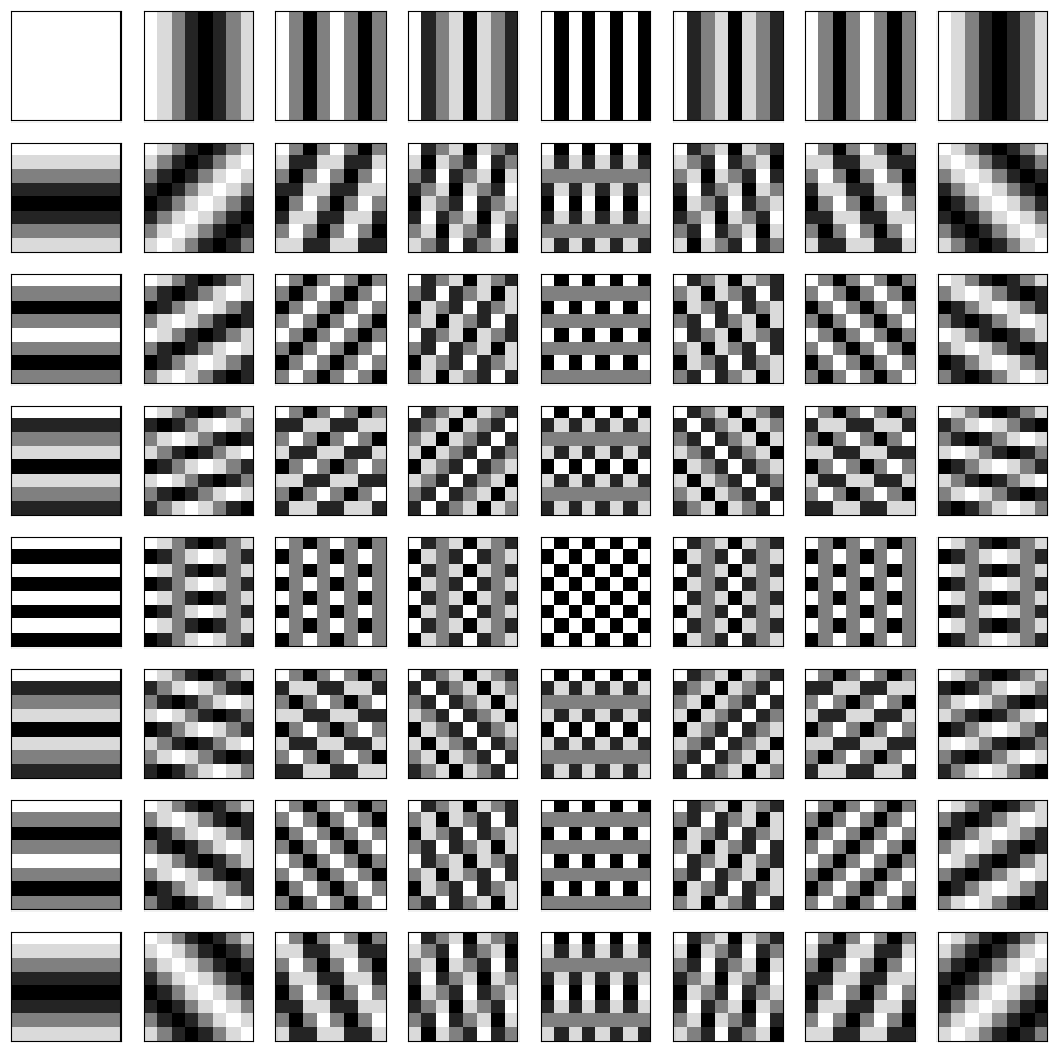

The discrete Fourier transform can be performed by computing the linear combination of the pixel values in the original image with the corresponding basis images.

Implementing DFT using such linear combination is computationally expensive, so let us limit ourselve to an image of size for now.

url = "https://www.cs.montana.edu/courses/spring2005/430/lectures/06/programs/checker32.jpg"
img = Image.open(requests.get(url, stream=True).raw).convert("L").resize((4, 4))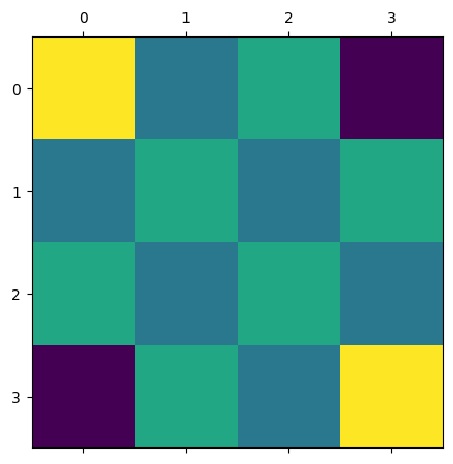

Since the image is of size , there will be 16 basis images.

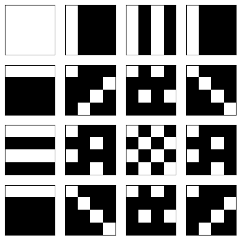
Then the Fourier transform can be performed using the linear combination discusses earlier as shown below

M, N = 4, 4
bases = [dft_bases_2d(M, N, i, j) for j in range(M) for i in range(N)]
bases_np = np.stack(bases, axis=2)

img_dft2_lin_comb = (img_np.reshape(1, 1, -1) * bases_np).sum(axis=2).reshape(4, 4)

plt.matshow(np.log(np.abs(img_dft2_lin_comb)**2))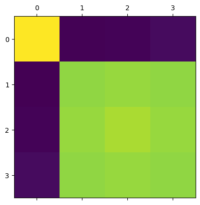

Let us again compare it with the fast Fourier transform from numpy to verify that it is correct.

print(np.isclose(img_dft2_lin_comb, np.fft.fft2(img_np)).all())

np.True_

This means that our implementation is correct.

References

• https://math.stackexchange.com/questions/1113398/discrete-fourier-transfomation-and-harmonics
• https://databookuw.com/